
The difference between probabilistic output vectors and target vectors is crucial for the network to learn. How can you measure this difference? What does the learning process look like? How do we indicate when our model is smart enough?
Previously, we ended with two vectors: the softmax vector and the target vector. The following one is the third part of Word2vec‘s description, so I strongly recommend getting acknowledged with the previous one before reading it.
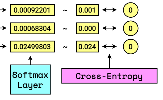
On the previous step, we had an output vector that is basically useless since it’s hard to interpret its components as indicators of the target word. That’s why we used the Softmax function. As a result, the output vector is transformed into a softmax vector and its sum of components equals one.

Now we can talk since the softmax vector stands for the probability distribution of the target word. Probability because in machine learning, we always work on controlled randomness. There is a chance for each one to appear. More about the relation between one-hot (“0-1-0”) vectors can be found in part no.1.
Cross-entropy
The target vector is the same type as the input vector: only zeros and a single ‘1’. In the meantime, output, softmax vector consists of everything but zeros and one. To compare them is crucial for indicating whether our network is doing a good job or failing. We will use cross-entropy for that.
Mode of action
[ {H(p,q)=-sum _{x} p(x) log q(x)} ]
So we have our target vector and softmax vector:
[ overrightarrow{V_T} = [1.0, 0.0, 0.0, 0.0, 0.0, 0.0] newline overrightarrow{V_S} = [0.411, 0.411, 0.151, 0.001, 0.000, 0.024] ]
We put them trough cross-entropy equation:
[ H(overrightarrow{V_T},overrightarrow{V_S}) = – [ overrightarrow{V_T} cdot ln ( overrightarrow{V_S} ) ] ]
[ H = – [ 0 cdot ln ( 0.411 ) + 1 cdot ln ( 0.411 ) + … + 0 cdot ln ( 0.024 ) ] ]
Notice that once again the one-hot vector acts as the pointer!
[ H = – [ 1 cdot ln ( 0.411 ) ] = 0.478]
Cross-entropy indicates how much network prediction is from the truth. What can we do with this knowledge?
Back Propagation: Stochastic gradient descent
For machines, learning means minimizing the value of error.
Our task is to find a minimum of the loss function. Neural networks update their weights to minimize the cross-entropy value. It cannot be easily visualized since, once again, we are talking about multidimensional space, but to understand the mode of action, we simplify it and present it in 3D space. Two dimensions for weights (two abstract values that we will adjust), and the third dimension for cross-entropy value.
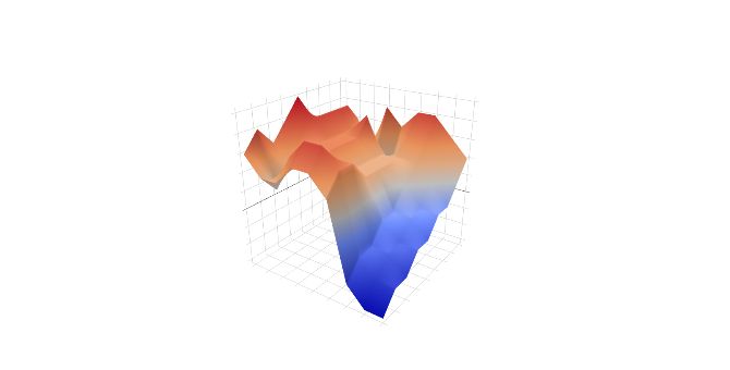
Optimization is about going down the hill of this surface since every combination of weights will give another output, so at the same time, another error value.
The lower we get “above mean sea level”, the closer we are to the right word prediction!
We are counting how far our prediction was from the truth, and updating values on nodes, to better express the actual state. This is more or less how the algorithm works. But sadly, it’s more prototype or proof of concept. In practice, word2vec is a bit more complicated.
This is only the beginning
The presented example is the simplest version of the already simple word2vec, focused on predicting words; in the meantime, we want to train the model, so more or less, we try to kill two birds with one stone. The presented learning model is highly inefficient due to the following reasons:
- One “round” is called an epoch. It covers processing over our network all of the training examples. For real-life examples where there are not six, but rather millions of words.
- Usually, there is more than one epoch in training. Much more.
- Along with the size of the vocabulary, dimensionality grows. Six, six-dimensional vectors are far easier to process than millions of thousands-dimensional vectors.
- Simultaneously, we calculate the probability of word occurrences and use this information to fix the network. It’s ok but works better as a polishing method, not necessarily an actual learning method.
In other words
The method we presented is about generating output and telling the machine whether it made wrong or bad decision. In fact, we are hoping for correct predictions and then forcing them through the network.
It’s like making a child perform math operations for the first time, watching it struggle, waiting, and saying in the end: “wrong, the correct answer is 5”. And so on, and so on. Not quite a wise pedagogical policy, is it?
Instead, we can show examples of correct and wrong answers without wasting time for calculations, knowing that the child/model is untrained. It’s called:
The Skip-Gram with Negative Sampling (SGNS)
Let’s show the machine a pair of words and instantly tell it if they appear in the same context or not!
If the words are paired, let’s label it with ‘1’. In this approach, as the input, we have two words (analyzed one and target word), and the output is the correct label. What about incorrect examples?
The wrong training answers (true negatives) are generated using a sample, analyzed word, and randomly chosen word that never appears in the context in the analyzed corpus.
Do you remember our tiny corpus from part 1?

So, the SGNS first training samples look like this. I’ve chosen 2 negative samples for each positive just to give you a glimpse of understanding. In fact the number of negative samples is, just like the frame size, a matter of analyst choice!

What to do next
We are about to use two matrices—one with embeddings, the second one with context. As always, in the beginning, we are filling them with random values. Don’t worry, they will be quickly adjusted!
- Embedding matrix – stands for the input words
- Context matrix – stands for the target words.
Let’s take a look at the first training three. What is happening right now?
- We pick embeddings (indicated by word vectors) from the embedding matrix and context matrix.
- We then count the dot product of them for each pair.
- We apply a logistic function to the result of the product. Doing so, we receive value from the range of 0 and 1.
- We subtract this value from the “Is Context” value (1 or 0)
- As a result, we receive an error added to the embedding values (both the input and the target) adjusting our network.
The process above is then repeated for each word training pair and then again (and again) over the whole vocabulary until we reach the desired precision. After we finish the pre-training process, we keep our embeddings matrix for further usage.
What we can do with it, we cover in the next episode!

Marcin Lewek
Marketing Manager
edrone
Digital marketer and copywriter experienced and specialized in AI, design, and digital marketing itself. Science, and holistic approach enthusiast, after-hours musician, and sometimes actor. LinkedIn