
People understand words with ease (usually). It’s a bit harder for computers, but we can represent words with numbers to make them comprehensive. Not just any numbers, but vectors. Surprisingly, it’s a common language for us, and that can lead to quite impressive things.
In the previous part, we learned how to turn words into vectors understandable for a machine. To be precise: able to be processed by machine relevantly and in a useful way. We didn’t mention it, but such transformation is called word embedding, as we embed these words in multidimensional space.
In this chapter, we are about to learn something about the process of finding relations, the affinity between words, and measuring this affinity.
Finding pairs
We’ve ended with a word-vector dictionary rooted in the tiny corpus of text:
'edrone is awesome'
'The First CRM for eCommerce and AI fueled marketing machine'
Each vector consists of a single ‘one’ and ten zeros. Each number stands for another dimension in 11-dimensional space. It means that each vector (One-hot Vector) is pointing exclusively in one and the only one dimension, which is, let’s say, its own.
{'ai':
 [0.0, 1.0, 0.0, 0.0, 0.0, 0.0, 0.0, 0.0, 0.0, 0.0, 0.0, 0.0, 0.0],

 'and':
 [0.0, 0.0, 0.0, 0.0, 0.0, 0.0, 0.0, 0.0, 0.0, 1.0, 0.0, 0.0, 0.0],

 'awesome':
 [0.0, 0.0, 0.0, 0.0, 0.0, 0.0, 0.0, 0.0, 1.0, 0.0, 0.0, 0.0, 0.0],

 'crm':
 [0.0, 0.0, 0.0, 0.0, 0.0, 0.0, 0.0, 0.0, 0.0, 0.0, 0.0, 1.0, 0.0],

 'ecommerce':
 [0.0, 0.0, 0.0, 1.0, 0.0, 0.0, 0.0, 0.0, 0.0, 0.0, 0.0, 0.0, 0.0],

 'edrone':
 [0.0, 0.0, 0.0, 0.0, 0.0, 0.0, 0.0, 0.0, 0.0, 0.0, 0.0, 0.0, 1.0],

 'first':
 [0.0, 0.0, 1.0, 0.0, 0.0, 0.0, 0.0, 0.0, 0.0, 0.0, 0.0, 0.0, 0.0],

 'for':
 [0.0, 0.0, 0.0, 0.0, 0.0, 0.0, 0.0, 1.0, 0.0, 0.0, 0.0, 0.0, 0.0],

 'fueled':
 [0.0, 0.0, 0.0, 0.0, 0.0, 1.0, 0.0, 0.0, 0.0, 0.0, 0.0, 0.0, 0.0],

 'is':
 [1.0, 0.0, 0.0, 0.0, 0.0, 0.0, 0.0, 0.0, 0.0, 0.0, 0.0, 0.0, 0.0],

 'machine':
 [0.0, 0.0, 0.0, 0.0, 0.0, 0.0, 1.0, 0.0, 0.0, 0.0, 0.0, 0.0, 0.0],

 'marketing':
 [0.0, 0.0, 0.0, 0.0, 0.0, 0.0, 0.0, 0.0, 0.0, 0.0, 1.0, 0.0, 0.0],

 'the':
 [0.0, 0.0, 0.0, 0.0, 1.0, 0.0, 0.0, 0.0, 0.0, 0.0, 0.0, 0.0, 0.0]}
Let’s use it in practice!
The more identical words appear in the same context as two chosen words, the more similar meaning they have. In the case of analysis, we use a strict definition of this closeness. It’s a frame of a given size. The frame’s size is optional, so let’s use the size of two. It means that we are going through text corpus, with the frame, writing down the words that appear before and after the analyzed piece, just like on the following scheme.
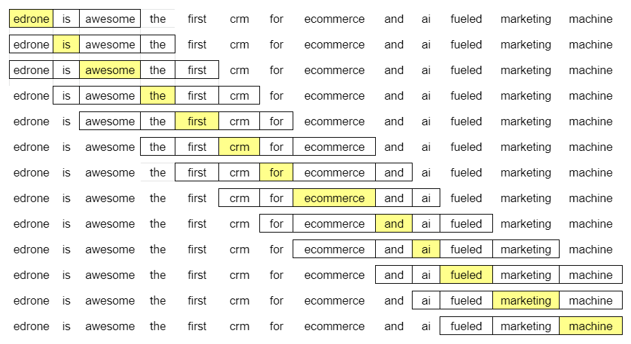
In line one, we have:
- (edrone, is)
- (edrone, awesome)
Later:
- (is, edrone)
- (is, awesome)
- (is, the)
And after that:
- (awesome, edrone)
- (awesome, is)
- (awesome, the)
- (awesome, first)
In fact, these pairs, translated for a machine language, look like this…
(edrone, is) ->
-> ([0.0, 0.0, 0.0, 0.0, 0.0, 0.0, 0.0, 0.0, 0.0, 0.0, 0.0, 0.0, 1.0],
    [1.0, 0.0, 0.0, 0.0, 0.0, 0.0, 0.0, 0.0, 0.0, 0.0, 0.0, 0.0, 0.0])
…and so on.
Our network’s task is to learn transformation that, with the left vector (upper on the example above) on the input, gives us the right vector (lower) on the output, which stands for the word with a similar meaning.
Input, hidden & output layer.
If you know something about Machine learning / Deep learning, you surely know or at least recognize a similar graph.
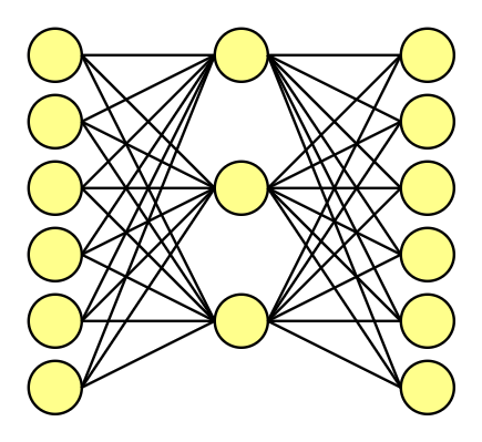
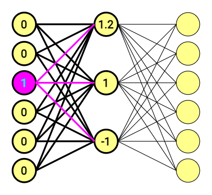
Let’s forget for a while about our previous vectors, and our tiny-test-corpus. This time, to better show the mechanics behind the neural network, let’s use a corpus of six original words. It’s much easier, to show how it works on a way smaller example.
So, we have six original words. What does it mean? That the word embedding vectors are 6-dimensional, consisting of 5 x zeros and 1 x one. We decide to use the hidden layer consisting of three nodes (just like size of the frame, it’s our subjective choice.)
When training this network on word pairs, the input is a one-hot vector representing the input word, and the training output is also a one-hot vector representing the output word.
But when you evaluate the trained network on an input word, the output vector (raw output, not the training output) will actually be a probability distribution (i.e., a bunch of floating-point values, not a one-hot vector). Still, we’ll come back to the output later.
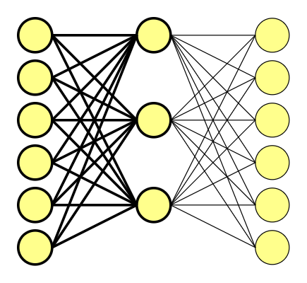
The first half of the scheme above translated into a mathematic equation looks like this.
[ begin{bmatrix} 0 & 0 & 1 & 0 & 0 & 0 end{bmatrix} times begin{bmatrix} 1 & 2 & 2\ -1 & 0 & -2\ 1.2 & 1 & -1\ -0.5 & -1 & 2\ -1 & 0 & -1\ 1 & 2 & -1 end{bmatrix} =begin{bmatrix} 1.2 & 1 & -1 end{bmatrix} ]
Matrix stands for connections between nodes – weights. These was also chosen at random, just an an example.
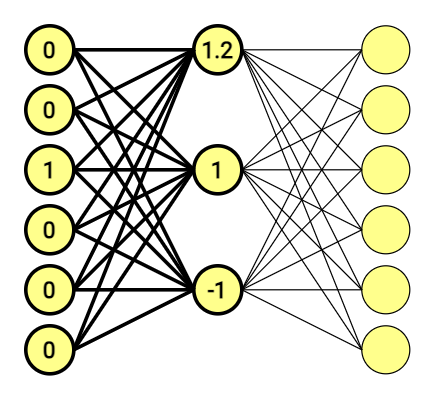
If you are proficient with linear algebra, you are probably asking yourself: “Wait a sec… if this vector is made of almost zeros, that means that I can compute it by just looking at it; where’s the catch?” If linear algebra and operations on vectors aren’t one of your feats, let me explain:
If you multiply a 1 x 6 one-hot vector by a 6 x 3 matrix, you will effectively just select the matrix row corresponding to the “1.0” in one-hot vector. And that’s it.

The one-hot vector consists of only one ‘1.0’ and zeros, for we are using it as the pointer. It also means that we are using a hidden layer as our lookup table.
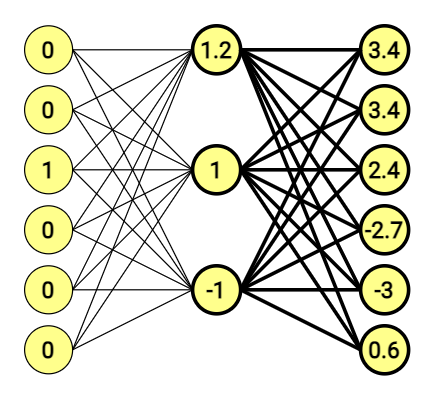
At the end of the day, we have 6-dimensional vectors on both sides. The second part of the equation looks similar, and is doing the same thing once again.

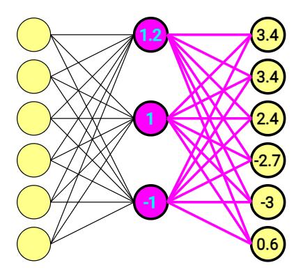
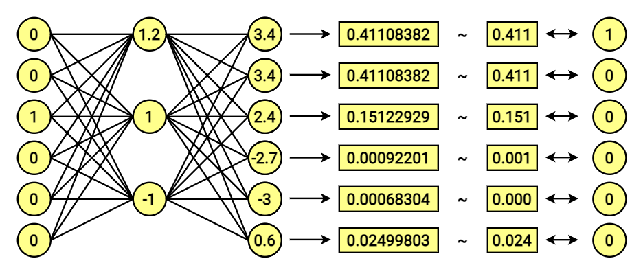
This time Output vector doesn’t look that clear, and – what is more important, doesn’t point at anything.
We are using the softmax function for that.
Softmax function:
[ {frac{e^{x}}{sum e^{x}}} ]
After aplication of softmax it becomes:
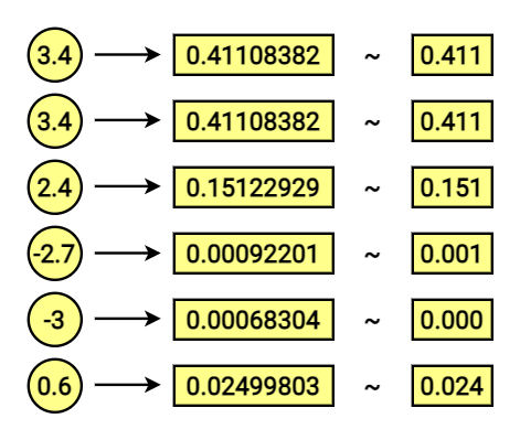
[0.41108382 0.41108382 0.15122929 0.00092201 0.00068304 0.02499803]Let’s transpose it for a better view:
[0.41108382
0.41108382
0.15122929
0.00092201
0.00068304
0.02499803]Notice that sum of its features equals 1!
The effect is the vector consisting of probabilities for corresponding dictionary vectors. In other words; The first number is the probability, for the output word being the first in our dictionary (corresponding to the [1,0,0,0,0,0] vector). The second stands for the second, and so on.
The difference between probabilistic output vector and target vector is crucial for the network to learn. We will learn more about this later.
Two approaches of word2vec
It’s the right moment to mention that two main approaches come with Word2vec: Continous Bag of Words (CBOW) and Skip-Gram. Long story short:
- CBOW – predicts central word, basing on surrounding words.
- Skip-Gram – indicates the context (surrounding words) using selected, single words.
As an example we used Skip-Gram. One once vector in the output, and matching it with one of the 4 training output vectors.
Which technique to use? Well, it depends on what exactly you want to achieve. Nonetheless, the architecture of our networks will look similar. The difference lays in which side of our pairs set we are about to use as an input and then respectively second as the feedback.
How to apply this feedback? What’s, is Loss function?
We’ll learn in part three!

Marcin Lewek
Marketing Manager
edrone
Digital marketer and copywriter experienced and specialized in AI, design, and digital marketing itself. Science, and holistic approach enthusiast, after-hours musician, and sometimes actor. LinkedIn